AI-Powered DEX Arbitrage Bots

Since my time at Deutsche Bank, I’ve been programming financial indicators, trading strategies, and arbitrage bots.
The early days were simple: indicators with alert systems that triggered notifications when specific conditions were met. I executed trades manually, which worked for long-term investments where speed wasn’t critical — at least for a while.

Later, in crypto, my approach to algorithmic trading evolved dramatically. By exploiting market imbalances between centralized exchanges like Poloniex and Bitfinex, I managed to run a fairly profitable arbitrage bot from a Raspberry Pi plugged into my home router. It was a different beast entirely, for several reasons:

• Live trading is far more complex than backtesting. Beyond spotting opportunities, you must manage liquidity and position sizing carefully.
• APIs are unreliable. They can go down, respond slowly, or return garbage data — and you need to be ready for all of it.
• Latency is everything. It became less about crafting clever indicators and more about spotting imbalances fast enough to act before the opportunity vanished.

That was the era of hardcoded rules, if-else statements, and relentless trial and error. Then came decentralized exchanges (DEXes) and liquidity pools — and the game changed again.

I began crafting a strategy based on deterministic logic to identify arbitrage opportunities across DEX pools. The idea was to use a mathematical model to detect imbalances — sometimes several hops away. My initial logic was primitive, and brute-force analysis soon became infeasible as the number and complexity of DEXes grew. I had to level up.

That’s when I started exploring machine learning, using TensorFlow to detect arbitrage patterns in market data. The idea was to leverage deep neural networks and reinforcement learning to uncover signals I’d otherwise miss. This changed everything. The model learned over time and spotted opportunities I would’ve never considered. Ignoring challenges like front-running, MEV, or gas fees — it was a promising direction.

While my current research has moved beyond simple DEX arbitrage, let me walk you through an experiment involving a transformer-based setup (yes, the same architecture powering today’s LLMs) applied to V2 pools, and why its performance shifts when applied to V3 pools.

V2 Pools

Before diving into transformers and their relevance to arbitrage, let’s revisit the mechanics of V2-style DEX pools, like those introduced by Uniswap V2. Understanding their deterministic nature is key to seeing how arbitrage opportunities emerge — and why they were once relatively easy to model.

A V2 liquidity pool operates as a constant product market maker (CPMM), where two tokens — say, token ( X ) and token ( Y ) — are pooled. The core invariant is:

$$x \cdot y = k$$

Where:

• ( x ) = reserve of token ( X )
• ( y ) = reserve of token ( Y )
• ( k ) = constant invariant

This formula ensures every trade preserves the product of reserves. For instance, swapping in some token ( X ) will return an amount of ( Y ) such that the new product ( x' \cdot y' = k ). In practice, fees slightly shift the invariant.

A Simple Arbitrage Opportunity

Let’s imagine two DEXes, DEX A and DEX B, each offering an ETH/USDC pool. Due to asynchronous trades, ETH might be priced at $1,950 on DEX A and $2,000 on DEX B.

Here’s a classic arbitrage sequence:

1. Buy ETH on DEX A for $1,950 USDC.
2. Sell the same ETH on DEX B for $2,000 USDC.
3. Profit: $50 (minus gas fees and slippage).

Because V2 math is fully transparent and deterministic, such cross-exchange arbitrage is easy to simulate and reason about.

Flash Loans (and Why You Might Not Need Them)

Flash loans are a clever DeFi primitive that let you borrow funds without collateral — as long as you repay them within the same transaction. In arbitrage, they’re handy when you don’t want to risk your own capital.

However, in circular arbitrage within DEXes (e.g., ETH → DAI → USDC → ETH), you often don’t need a flash loan if the opportunity is contained within a single atomic transaction — just initial capital and good execution.

What made V2 special was its predictability. Every quote could be computed off-chain. Every route pre-simulated. It was fertile ground for rule-based bots, early ML models, and eventually, transformer-based agents.

Modern Transformer Architecture

Simulating a multi-DEX, multi-pool environment is relatively easy. You can customize token amounts, pool sizes, connection densities, flash loan providers, and inject arbitrage opportunities with varying frequency. This creates an ideal environment for training transformer-based models on virtually unlimited data.

My recent setup differs from past approaches. The focus was on testing how modern transformer architecture — inspired by LLMs — performs in this context.

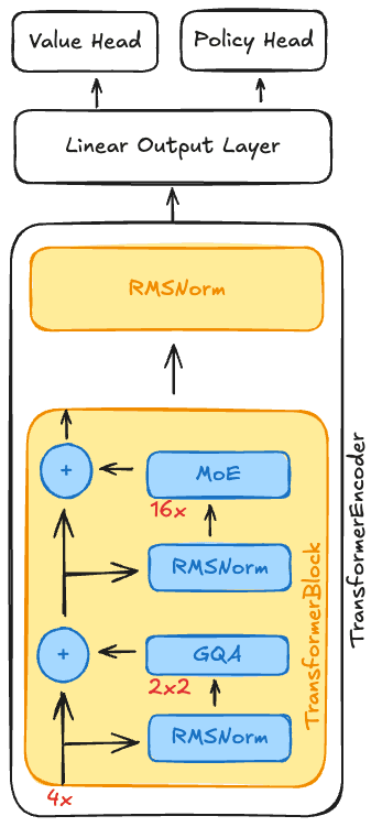
The network consists of a Transformer Encoder, followed by a Linear Output Layer, split into PPO-style heads (value and policy) for prediction. The encoder includes 4 stacked Transformer Blocks, ending with a final RMS Normalization Layer.

You’ll notice there’s no token embedding layer. All encodings were handcrafted — I’ll explain why in the I/O section.

GQA: Grouped-Query Attention

Each Transformer Block includes a Grouped-Query Attention mechanism with 4 attention heads divided into 2 groups. While 4 heads aren’t computationally heavy, I wanted to experiment with this recent improvement.

MoE: Mixture of Experts

The expert layer uses a linear router and 16 SwiGLU Feedforward “Experts”. For each token, three experts are dynamically selected, and a fourth is an always-on generic expert.

All results are passed through RMS Normalization, then merged and fed into the next block. This process repeats through the 4 layers until the final output.

Input and Output

AI is no magic bullet — it requires thoughtful planning and design. The success of the model hinges on well-structured inputs and outputs.

In LLM pretraining, you often start with large datasets and random embeddings. In this case I wanted to have clear embeddings right from the start, so I engineered a custom encoding scheme:

The DEX pools can be represented as a graph, where nodes are tokens and edges are liquidity pools. I could encode each token as a normalised one-hot vector, and each pool as a sum of its two token vectors, weighted by their reserves. This way, the model can easily learn relationships between tokens and pools.

For example, consider three tokens: ETH, USDC, and DAI. Their one-hot encodings might look like this:

$$\mathbf{eth} = [1, 0, 0, \ldots, 0] \\ \mathbf{usdc} = [0, 1, 0, \ldots, 0] \\ \mathbf{dai} = [0, 0, 1, \ldots, 0] \\ \ldots \\ \mathbf{etc} = [0, 0, 0, \ldots, 1]$$

I selected a big enough vector size (e.g., 128 dimensions) to allow adding new tokens, even if my initial set consisted of only a few dozen tokens and their pools. The pool encoding for a eth/usdc pool with reserves $\mathbf{eth}$ and $\mathbf{usdc}$ would be:

$$\mathbf{pool}_{eth/usdc} = [100, 400000, 0, \ldots]$$

Where 100 is the amount of ETH and 400,000 is the amount of USDC in the pool.

Now, each of those pool vectors were extended with additional features:

• 6 dimensions: DEX id (one-hot, supports up to 6 DEXes)
• 1 dimension: Pool fee tier (percentage per swap)
• 2 × 2 dimensions: Lending info (AAVE): available liquidity and supply rate for both tokens

Hence, the final input vector dimension for each pool becomes:
$128 + 6 + 1 + 4 = 139$ dimensions.

The beauty of these manual embeddings and orthogonality of the one-hot vectors is that the model can easily learn relationships between tokens and pools without needing to learn embeddings from scratch.

My final input matrix had a fixed size as well — similar to the input context length in LLMs. I set a maximum number of pools (e.g., 50), and if there were fewer pools, I padded the input with zero vectors. This ensured consistent input dimensions for the transformer.

Example matrix with $n$ where $n \leq 50$ pools:

$$\mathbf{input} = \begin{bmatrix} \mathbf{pool}_1 \\ \mathbf{pool}_2 \\ \vdots \\ \mathbf{pool}_{n} \\ \mathbf{zero}_{n+1} \\ \vdots \\ \mathbf{zero}_{50} \\ \end{bmatrix}$$

No positional encodings

Since the order of pools in the input matrix is arbitrary (unlike words in a sentence), I did not include positional encodings. The transformer’s self-attention mechanism can learn relationships between pools regardless of their order.

Output

The policy head output was a single vector of the following structure:

$$\mathbf{output} = [amount_{in}, token_{start}, token_{hop1}, token_{hop2}, \ldots]$$

Where:

• $\mathbf{amount_{in}}$ = investment amount of the starting token
• $\mathbf{token_{start}}$ = starting token id (positional index of the one-hot vector)
• $\mathbf{token_{hop1}}$ to $\mathbf{token_{hopN}}$ = next token ids

The output dimensions were fixed to 10, allowing up to 8 hops. To signal early stopping, the network returned a negative value as a token id. All following hops were ignored in simulation.

Training and Results

I used the simulator to generate DEXes with different amounts of pools, tokens, and connection densities. I injected arbitrage opportunities at random intervals, varying their frequency and complexity. I simulated real-world conditions for gas fees, slippage, and flash loan requirements.

The model was trained using Proximal Policy Optimization (PPO), a reinforcement learning algorithm well-suited for continuous action spaces. The reward function was based on the profit generated from executed arbitrage trades, minus gas fees and slippage.

Training was done in episodes, where each episode consisted of a fixed number of simulation steps. At each step, the model observed the current state of the DEX pools, made a decision based on its policy, and received a reward based on the outcome of that decision.

After training for about 3–4 million episodes, the model was able to identify and execute arbitrage opportunities with a high degree of accuracy. It achieved a significant increase in profit compared to the baseline (brute-force strategy), demonstrating the effectiveness of the PPO algorithm in combination with my transformer-based architecture in this context.

It could identify complex arbitrage paths — sometimes different (but more profitable) than the injected imbalance — showing an emerging behaviour that adapted to new market conditions.

Final success rate: 98.9% on the test set.

V3 Pools

V3 pools introduced a new level of complexity with their concentrated liquidity and multiple fee tiers. Unlike V2, where liquidity is uniformly distributed across the price curve, V3 allows liquidity providers to concentrate their liquidity within specific price ranges. This fundamentally changes the dynamics of how trades impact pool reserves and, consequently, how arbitrage opportunities arise.

It also made the simulation and prediction task significantly harder. In the end, I have used a rule-based approach to achieve similar performance as with V2 pools — without training and without computational overhead.

This showed once again that not everything should be solved with machine learning. Sometimes, a well-crafted algorithmic solution is more efficient and effective.

I’ll explain the V3 approach in a future article.

Conclusion

The experiment with transformer-based arbitrage bots in a simulated DEX environment yielded promising results, especially with V2 pools. The model demonstrated a strong ability to identify and exploit arbitrage opportunities, achieving a high success rate.

This is also the basis of my current research on using transformers for more complex DeFi strategies using other primitives apart from the DEX pools — such as principal/yield splits, hedging yields, and more - where the deterministic approach might not suffice.